Category Archives: Stock Market

NIKKEI 225 Break Analysis…Overdone ?

In the following I us an R package BFAST designed to detect strucutural breaks in time series.The script Iteratively detects breaks in the seasonal and trend component of a time series. The first chart shows the various break and fitted regressions. The second chart shows the deviations from the regression lines and 95% interval of confidence. This could be used as an overbought/oversold indicator. Anyway, just work in progress…so any input / suggestions are always welcome as usual. Feel free to contact me at:Pierre@argonautae.com

plot of chunk plot plot of chunk plot

Trade Weighted Currency Indices Stretch Map

Trade Weighted Currency Indices Report

Tue Dec 08 22:57:28 2015

The following report aims to provide a gauge to the current strenght of major currencies. For doing so I use the Bank of England Trade weighted Exchange rate indices and a standardised statistical measures of price deviation to provide an estimate of how stretched major currencies are on a trade weighted perspective.

plot of chunk linechart

I first calculate the T-stat of the mean price deviations over a rolling period of 61 days. The charts below show the results for each currency over the last 500 days. The purple line represents the median value since 1990-01-03 and the red lines represent the 95% confidence intervals. Therefore if the value is above or below those the deviation of the given currency would be deemed as atypical relative to what #would be expected under a normal distribution and therefore overbought/oversold.

plot of chunk rolling chart

The following Map chart shows how stretched the currencies are over time horizons ranging from 1-month to 1-year. The bigger the square the most significant the upside (green) or downside (red) of currencies over the given period.

plot of chunk stretch map
The charts below show how the daily changes in the Trade weighted indices have correlated since January 1990 and since the begining of 2015.

plot of chunk correlation
Finally, the following provide an ARIMA forecast for each of the trade weighted indices. My script selects the best ARIMA fit over the previous 250-day to generate a forecast for the next 21 days.
It also shows the forecast confidence intervals.

plot of chunk arimaforecastplot of chunk arimaforecastplot of chunk arimaforecast

Chinese Stock Market Risk Report Update

The following report provides an update on some of the metrics I use to classify market risk. The word classify is more appropriate as I think that in essence you cannot forecast risk but rather attempt to adjust to it into a timely fashion. Clearly risk would not be a risk if you could forecast it accurately. However as there is generally some degree of persistence in risk regimes, using a dynamic classification may be a useful approach for portfolio rebalancing and hedging. In this report I use the CBOE China ETF Volatility Index (VIX China) as a measure of stock market risk for China . The same methodology can be successfully applied to other inputs. Feel free to contact me at pollux@argonautae.com for more information on the subject.

In my approach I recognise that the nominal level of implied volatility is a crude metric of risk therefore I also use two other measures. The VIX Volga, a measure of uncertainty of risk and the ShockIndex a measure of market dislocation. VIX Volga is simply the volatility of the VIX China over a given period. This measure highlights how uncertain and unstable the level of risk has become. Though positively correlated to the level of the VIX China the VIX China Volga is not necessarily dependent on it. You can have a high level of volga whilst the VIX China is trading at rather innocuous levels. This is not a trivial observation as the leverage undertaken by market participants tends to be an inverse function of market volatility which implies a greater vulnerability when volatility becomes uncertain at low levels and therefore cannot be accurately budgeted fo r. The ShockIndex is the ratio between the Volga and VIX at the beginning the historical window chosen to evaluate the Volga. It quantifies sharp changes and acceleration in risk levels. Historically it has proven to be a good classifying measure for market event risks.

The below charts shows those three measures both relative to a time axis and their historical distribution. The red lines are the 95% confidence intervals, the purple line the median. The blue line highlight the current level. The VIX Volga and ShockIndex in this report are evaluated over a period of 14 days. The medians and 95% confidence intervals are calculated over the full history going back to 1990 though the charts shows only the recent years.

plot of chunk riskchart

At close of business the 2015-12-07 the VIX China was trading at 28 at the 67.2 percentile. The 14-day VIX China Volga was estimated at 12.4 its 41.4 percentile and the China shockindex at 0.4 or its 28.5 percentile.

The above charts are useful, however their visualisation is quite limiting. On the one hand we need quite a few charts to present the data on the other hand it is difficult to show the full VIX history going back to 1990 as this would make the charts unreadable. Therefore clustering and aggregating the whole data into a single chart should be useful to the end user. To answer this I use a mapping technique developed by Kohonen in the 1980′. It uses an unsupervised neural network to re-arrange data around meaningful clusters. Though computationally complex is a practical way to summarise multidimensional data into a low (usually 2) dimensional system.

The below chart shows how the VIX price history was split into 4 distinct clusters. Those clusters where computed not only as a function of the VIX level but also as a function of the other variables, namely VIX volga and Shockindex.

Since 03/2011 the VIX China traded 44 % of the time in Cluster 1, 39 % in Cluster 2, 11 % in Cluster 3 and 6 % in Cluster 4. Overall the layering provided seems quite intuitive as the increase in risk and time spent in each cluster points toward what would generally be expected from market risk regimes ranging from low to high risk.

plot of chunk cluster_chart

In the chart below we zoom on the various regimes within which the VIX has been trading for the current year. so far it traded 67 % of the time in Cluster 1, 33 % in Cluster 2, 0 % in Cluster 3 and 0 % in Cluster 4.

plot of chunk ytdriskchart

Finally the below chart shows a Self Organising Map of the above mentioned risk metrics. The data has been grouped and colored as a function of four clusters of increasing market risk regimes. Obviously as shown on the map, the minimum level of volatility pertains to cluster 1 and the highest to cluster4. The current regime and its progression from 21 days ago is also highlighted on the map.

plot of chunk SOM_chart

Always happy to discuss any of the above, feel free to reach me at: pollux@argonautae.com

Chinese Stock Market Risk Report 09-06-2015

The following report provides an update on some of the metrics I use to classify market risk. The word classify is more appropriate as I think that in essence you cannot forecast risk but rather attempt to adjust to it into a timely fashion. Clearly risk would not be a risk if you could forecast it accurately. However as there is generally some degree of persistence in risk regimes, using a dynamic classification may be a useful approach for portfolio rebalancing and hedging. In this report I use the CBOE China ETF Volatility Index (VIX China) as a measure of stock market risk for China . The same methodology can be successfully applied to other inputs. Feel free to contact me at pollux@argonautae.com for more information on the subject.

In my approach I recognise that the nominal level of implied volatility is a crude metric of risk therefore I also use two other measures. The VIX Volga, a measure of uncertainty of risk and the ShockIndex a measure of market dislocation. VIX Volga is simply the volatility of the VIX China over a given period. This measure highlights how uncertain and unstable the level of risk has become. Though positively correlated to the level of the VIX China the VIX China Volga is not necessarily dependent on it. You can have a high level of volga whilst the VIX China is trading at rather innocuous levels. This is not a trivial observation as the leverage undertaken by market participants tends to be an inverse function of market volatility which implies a greater vulnerability when volatility becomes uncertain at low levels and therefore cannot be accurately budgeted fo r. The ShockIndex is the ratio between the Volga and VIX at the beginning the historical window chosen to evaluate the Volga. It quantifies sharp changes and acceleration in risk levels. Historically it has proven to be a good classifying measure for market event risks.

The below charts shows those three measures both relative to a time axis and their historical distribution. The red lines are the 95% confidence intervals, the purple line the median. The blue line highlight the current level. The VIX Volga and ShockIndex in this report are evaluated over a period of 14 days. The medians and 95% confidence intervals are calculated over the full history going back to 1990 though the charts shows only the recent years.

plot of chunk riskchart

At close of business the 2015-06-08 the VIX China was trading at 32.3 at the 86.9 percentile. The 14-day VIX China Volga was estimated at 12.3 its 42.5 percentile and the China shockindex at 0.4 or its 19.8 percentile.

The above charts are useful, however their visualisation is quite limiting. On the one hand we need quite a few charts to present the data on the other hand it is difficult to show the full VIX history going back to 1990 as this would make the charts unreadable. Therefore clustering and aggregating the whole data into a single chart should be useful to the end user. To answer this I use a mapping technique developed by Kohonen in the 1980′. It uses an unsupervised neural network to re-arrange data around meaningful clusters. Though computationally complex is a practical way to summarise multidimensional data into a low (usually 2) dimensional system.

The below chart shows how the VIX price history was split into 4 distinct clusters. Those clusters where computed not only as a function of the VIX level but also as a function of the other variables, namely VIX volga and Shockindex.

Since 03/2011 the VIX China traded 55 % of the time in Cluster 1, 31 % in Cluster 2, 9 % in Cluster 3 and 5 % in Cluster 4. Overall the layering provided seems quite intuitive as the increase in risk and time spent in each cluster points toward what would generally be expected from market risk regimes ranging from low to high risk.

plot of chunk cluster_chart

In the chart below we zoom on the various regimes within which the VIX has been trading for the current year. so far it traded 77 % of the time in Cluster 1, 23 % in Cluster 2, 0 % in Cluster 3 and 0 % in Cluster 4.

plot of chunk ytdriskchart

Finally the below chart shows a Self Organising Map of the above mentioned risk metrics. The data has been grouped and colored as a function of four clusters of increasing market risk regimes. Obviously as shown on the map, the minimum level of volatility pertains to cluster 1 and the highest to cluster4. The current regime and its progression from 21 days ago is also highlighted on the map.

plot of chunk SOM_chart

Always happy to discuss any of the above, feel free to reach me at: pollux@argonautae.com

S&P500 Update…

Whatever the market being traded, there always will be a a question being asked at one moment: How far can this thing go ? Clearly not an easy question to answer as this will invariably depends on factors that are partly unknown or difficult to estimate, such as fundamentals, market positioning or market risk amongst others. The first part is obviously to assess how atypical the move experienced in the given instrument is. This report aims to contribute to this.

The below chart shows the S&P 500 over the period of January 1950 to June 2015 . On the 08 June 2015 it was trading around 2079.28003.

plot of chunk chartdata

In the below I plot the previous 125 days against other similar historical periods that would have closely matched the recent history. The data has been normalised so as to be on the same scale. The chart shows the latest 125 days in black, and overlay similar historical patterns in grey. It Also shows what has been the price path for the following 125 days as well as the observed quartiles.

plot of chunk pattern

Finally I plot the last 125 days and a trend forecast derived from an ARIMA(3,0,2) model as well as the 95% confidence intervals. The ARIMA model is fitted to the past 625 historical values whilst ignoring the last 125 days, therefore we can look at the recent price path against the trend forecast and its confidence intervals to gauge how (a)typical the recent move has been.

plot of chunk arimaplot

Brazil Stock Market Risk Report 09-06-2015

Ok it seems that I have a few Brazilian followers so I thought that I would produce something specific to Brazil…

The following report provides an update on some of the metrics I use to classify market risk. The word classify is more appropriate as I think that in essence you cannot forecast risk but rather attempt to adjust to it into a timely fashion. Clearly risk would not be a risk if you could forecast it accurately. However as there is generally some degree of persistence in risk regimes, using a dynamic classification may be a useful approach for portfolio rebalancing and hedging. In this report I use the CBOE Brazil ETF Volatility Index (VIX Brazil) as a measure of stock market risk for Brazil . The same methodology can be successfully applied to other inputs. Feel free to contact me at pollux@argonautae.com for more information on the subject.

In my approach I recognise that the nominal level of implied volatility is a crude metric of risk therefore I also use two other measures. The VIX Volga, a measure of uncertainty of risk and the ShockIndex a measure of market dislocation. VIX Volga is simply the volatility of the VIX Brazil over a given period. This measure highlights how uncertain and unstable the level of risk has become. Though positively correlated to the level of the VIX Brazil the VIX Brazil Volga is not necessarily dependent on it. You can have a high level of volga whilst the VIX Brazil is trading at rather innocuous levels. This is not a trivial observation as the leverage undertaken by market participants tends to be an inverse function of market volatility which implies a greater vulnerability when volatility becomes uncertain at low levels and therefore cannot be accurately budgeted fo r. The ShockIndex is the ratio between the Volga and VIX at the beginning the historical window chosen to evaluate the Volga. It quantifies sharp changes and acceleration in risk levels. Historically it has proven to be a good classifying measure for market event risks.

The below charts shows those three measures both relative to a time axis and their historical distribution. The red lines are the 95% confidence intervals, the purple line the median. The blue line highlight the current level. The VIX Volga and ShockIndex in this report are evaluated over a period of 14 days. The medians and 95% confidence intervals are calculated over the full history going back to 1990 though the charts shows only the recent years.

plot of chunk riskchart

At close of business the 2015-06-05 the VIX Brazil was trading at 31.6 at the 65.6 percentile. The 14-day VIX Brazil Volga was estimated at 10.7 its 17.3 percentile and the Brazil shockindex at 0.3 or its 6.3 percentile.

The above charts are useful, however their visualisation is quite limiting. On the one hand we need quite a few charts to present the data on the other hand it is difficult to show the full VIX history going back to 1990 as this would make the charts unreadable. Therefore clustering and aggregating the whole data into a single chart should be useful to the end user. To answer this I use a mapping technique developed by Kohonen in the 1980′. It uses an unsupervised neural network to re-arrange data around meaningful clusters. Though computationally complex is a practical way to summarise multidimensional data into a low (usually 2) dimensional system.

The below chart shows how the VIX price history was split into 4 distinct clusters. Those clusters where computed not only as a function of the VIX level but also as a function of the other variables, namely VIX volga and Shockindex.

Since 03/2011 the VIX Brazil traded 42 % of the time in Cluster 1, 41 % in Cluster 2, 10 % in Cluster 3 and 6 % in Cluster 4. Overall the layering provided seems quite intuitive as the increase in risk and time spent in each cluster points toward what would generally be expected from market risk regimes ranging from low to high risk.

plot of chunk cluster_chart

In the chart below we zoom on the various regimes within which the VIX has been trading for the current year. so far it traded 45 % of the time in Cluster 1, 38 % in Cluster 2, 4 % in Cluster 3 and 12 % in Cluster 4.

plot of chunk ytdriskchart

Finally the below chart shows a Self Organising Map of the above mentioned risk metrics. The data has been grouped and colored as a function of four clusters of increasing market risk regimes. Obviously as shown on the map, the minimum level of volatility pertains to cluster 1 and the highest to cluster4. The current regime and its progression from 21 days ago is also highlighted on the map.

plot of chunk SOM_chart

Always happy to discuss any of the above, feel free to reach me at: pollux@argonautae.com

US MUTUAL FUND FLOWS REPORT UPDATE 18-02-2015

Wed Feb 18 15:30:28 2015

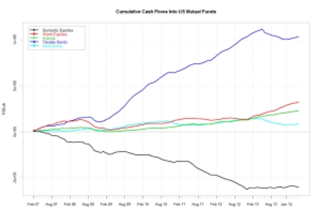
Fund flows are important as they reflect the general investor preference for a specific asset class given current and expected economic conditions and market risk. They may also highlight non-sustainable market positioning. The ICI in the US tracks about 98% of the inflows and outflows in US mutual funds and makes its data freely available on its website. The following is a summarised report of the data it publishes every Wednesday. The first charts shows the cumulative inflows/outflows in each of the asset classes buckets since 2007

plot of chunk cumulative

During the month of February we have seen flows of US$ 3.51Bn in Domestic equities,US$ 2Bn in international equities, US$ 1.75Bn in Hybrid products,US$ 7.44 Bn in taxable bond funds and US$ 1.66Bn in non taxable bond funds.

plot of chunk month to date The Charts below shows the distribution in percentage terms of the US$ 63Bn that have flowed into US$ Mutual funds over the last 12-month.

plot of chunk distribution

The below charts show the monthly inflows/outflows for each type of fund and plot them both within their 95% confidence intervals and also relative to their historical distribution. This provides a level of information in respect of how “out of line” or not the current month inflows/outflows may be relative to their past history. In the distribution charts The current month is highlited in blue whereas the vertical red lines represent the 95% confidence intervals.

plot of chunk flowdistribution

The chart below plot the inflows/outflows T-statistics for each of the funds cathegories considered. The Map chart provides information for period ranging from 2 years to 3 months.The greater the square the more important the inflows (green) outflows(red) over a given period.

plot of chunk flowmap

Is The Fed Changing Its View About Inflation ?

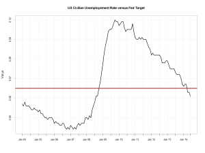
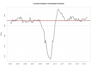
Yesterday in her  Semi-annual Monetary Policy Report to the Congress,  Chairman  Janet Yellen  stated the following: “If the labor market continues to improve more quickly than anticipated by the Committee… then increases in the federal funds rate target likely would occur sooner and be more rapid than currently envisioned.”  However Treasury yields  have barely moved and the dollar appreciation  again the Greenback remained muted . The Euro depreciated only by 0.6% against the US Dollar since her speech.  As shown from the chart below though the dollar against a broad basket of currencies is fairly well priced this is not the case for 10-year yields. US 10 year yierld traded weighted Against all odds, Yellen  seems to have managed to contain market expectations yet again. This is quite outstanding when one looks at the hard data. Unemployment is clearly below the 6.5%  Fed target level. Also the rise in industrial production is quite telling of  an even lower unemployment rate in the months to come. unemployement USINDPRO

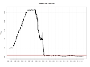
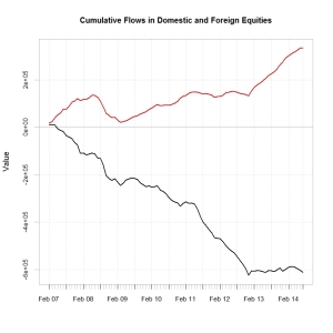
It is true that we have not yet seen much wage inflation in the us. The annual rate of increase in the average hourly earnings remains below 2% as shown below.  Wages remain dampened by the spare labour capacity. average earnings Clearly the Fed has accepted to remain behind the curve for quite a while  so  as not  to compromise any renewed  growth  in the US. The current low level of the Fed fund rate is a good illustration of  this. Fed Fund Contributing to a generally  dim view on the US economy by Fed members  could be that many forecasting models use 2×10 spreads as an input to forecast GDP. The abnormally ultra-low fed fund and therefore current steepness of the curve  could contribute to why  the Fed  growth forecasts may not be as accurate as should be.  After all even the IMF got it wrong with its growth forecast for the UK. 2x10It is now noticeable that over the last few months,  Inflation has crept  above the 2% target of the fed as indicated by the below chart. This is not surprising as trend in consumerism and aptitude of  price increase  is somehow function of  employments and wages earned. Though arguably not yet at an alarming level it will be interesting to watch out how the Fed react to further developments. US CPI So is the Fed starting to worry about inflation ? Plotting a Word Cloud of Yellen’s  speech it is indeed quite clear that Inflation is the central issue …..   yellen speechBearing in mind the above  it will be interesting to watch out for changes in the pattern of the inflows/outflows in US mutual funds. My thought is that we could see a resuming of the exit of bond products which was compromised by the ultra dovish tone adopted by Yellen when she took office. As mentioned in my previous post , the relative inflow/outflow in US versus foreign equities  could also have a perverse effect on the valuation of the US Dollar. High rates are not necessarily a long term driver of currency , capital flows are more important.  As a remainder of the current trends in US mutual funds  below are  couple of charts of my previous post. They show the distribution of the inflows/outflows in US mutual funds by asset class since the beginning of the year and the cumulative   flows in domestic versus foreign equities products since 2007. distribution inflows 2014cumulative flows I’ ll stick to my Long global equities and short dollar view…..

US Mutual Funds Flows Update: Investors Still Favouring International Equities

As it has been a while  since I have posted something and my broken arm is no longer a valid  excuse , I thought I would provide an update on  trends  in US mutual funds flows. To my surprise, bearing in mind the current geopolitical risks,  there has not been much change over the last few weeks. US investors have held onto  their preference for international equities whilst staying shy from the US stock markets. Also the trend of inflow into bonds   remained despite growing expectation of the Fed becoming more hawkish down the line. The map below shows the T-stats of the inflow/outflows across different time periods.

FLOWMAP

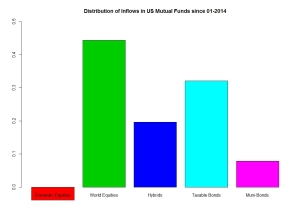
Clearly the dovish tone adopted by the Fed  has helped both the trend in equities and also bonds.  The question is how long  can this last ? Clearly the strengthening  observed in the US job market demonstrates that significant growth has rooted. Down the line this will create an issue for the fed, as managing rate expectations  whilst turning away from a dovish stance may prove challenging.  To me the most interesting point of all  is how US investors voted with their money. As can bee seen from the below charts they have stayed well away from US equities whilst investing in Foreign equities. In fact out of the US$ 133 bn invested in US mutual funds  44 %  (US$ 59 bn) went into  foreign equities  so far this year, whilst  US$ 5bn came out from US Stocks funds.

cumulative flows  distribution inflows 2014

As said in my previous posts I believe that what we are seeing could be a good explanatory variable as of  why the dollar has been so weak and particularly against the EURO despite the monetary expectation in Europe and the US. Bearing in mind the current market positioning and central bank flows it may well be that the  EURUSD is currently undervalued….


Long Equities as Usual

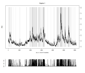
As market risk has been trading on the low over the last few months I thought that I would post a few charts of mine. First looking at the VIX as a measure of  financial market risk we are indeed trading at relatively low level, though we are still a few points away from the  9.31 the lowest ever close that printed on the 22nd of December 1993 .  The  two states Markov regime switching remains  clearly on risk seeking mode.

vixregime

Contributing to this low volatility has been the massive inflows that we have seen on equity markets.  However I would not call this level abnormal, the chart above  start from January 1990 and show that we have indeed experience long period of low volatility in the past. The chart below shows the significance of  inflows/outflows in US mutual funds tracked by the ICI . The chart on the left shows the T-stat of the inflows for the main asset classes over various time horizons. It is clear that the preference has been for  equities, and this with good reasons as discussed in my previous posts. So far in the US alone we have seen close to USD 120 billions of new inflows in US mutual funds.

flowmap05062014 inflow dist

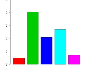
Out of this, as shown by the right hand chart,  close to 40% went into Foreign equities , only 5% into US equities and   21% in hybrids. if we assume a 60/40 benchmark this means an extra 8% into equities. Therefore  potentially 53% of the 120bn invested went into equities.  This is somehow in decline in respect of what we have seen in the first half of 2013 where 162bn went into US mutual funds, with an estimated 62%allocated to equities.  However this is without any doubt a contributing factor to the low level observed in the VIX. Clearly central banks monetary policy  and also the implication for the bond market of an exit scenario on the back of better economic fundamentals has somehow  been behind the great rotation that started now a couple of years ago. The last chart showing the cumulative inflows in the main asset classes indicates that  there is still some way to go….I ll stick to equities as usual….

cumulative